Blob Analysis

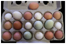
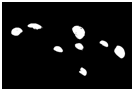
A group of connected pixels is commonly called a blob. Here is an example of an image containing a few blobs. The original image is segmented and the connected components are determined and visualized by color.

Original Image	Segmented Image	Connected Components

Blob analysis takes a set of connected pixels that are usually generated by imaging real-life objects, and calculates features from the pixel set, such as their area, their position, etc.

Often blobs are produced by some segmentation process, and one of the simplest segmentation methods is binary thresholding: every pixel with a value below the threshold is part of the background and every other pixel is part of some blob. Exactly which blob the pixel is a part of is determined by a connectivity analysis process sometimes called labelling or connected components analysis.

The smallest possible blob consists of a single pixel, and larger blobs consist of several connected pixels.

Does this picture contain one or two blobs?

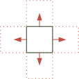
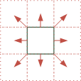
Have a look at the image above: Does this picture contain one or two blobs? It depends on how you look at it. If you only allow connections via horizontal and vertical neighbours, the picture contains two blobs. However, if diagonal connections count as well, the picture contains one blob only.

4-connected	8-connected

By convention, one often uses 8-connectedness for the foreground and 4-connectedness for the background pixels. According to this convention, the following picture contains one white object with two black holes.

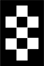
One white object with two black holes

One can summarize the relations of the above picture with the following table.

The table clearly shows that there are only two useful connectivity configurations:

Foreground Connectivity	Background Connectivity	Objects / Holes
4	4	7 / 2
4	8	7 / 0
8	4	1 / 2
8	8	1 / 0

• One (white) object with two (black) holes, or
• Seven (white) objects with no holes.

The other possible configurations do not make any sense, regardless how you look at them.

By default, nVision assumes that foreground pixels are 8-connected and background pixels are 4-connected.

nVision uses regions to represent blobs. Blob analysis is then the process of calculating region features. Because of the efficient run-length storage of regions, these features can be calculated very quickly. Since a region does not contain any pixel values, region features do not need to touch pixels. For a surprisingly large number of features pixel values are not necessary, such as the area or the center of gravity. Here is an example of how a region_list can be created by thresholding and connected components analysis:

Semgmentation, connected components analysis and blob analysis.

However, there is also a class of features that can only be calculated when you take pixel values into account, such as the mean brightness of a blob. nVision has a set of functions that can calculate pixel based features as well, but keep in mind that the performance requirements of calculating these features are higher. For pixel-based features, you still need a region to specify the object.

Here is a list of the region features:

Feature	Description
Area	The area as a number of pixels.
Left	The leftmost column position (inclusive).
Right	The rightmost column position (exclusive).
Top	The topmost row position (inclusive).
Bottom	The bottommost row position (exclusive).
Width	The width (axis parallel).
Height	The height (axis parallel).
Aspect Ratio	The axis parallel aspect ratio.
Bounds	The axis-parallel bounding box.
Perimeter	The perimeter.
Compactness	The compactness.
Circularity	The circularity.
Sphericity	The sphericity.
Roughness	The roughness.
Roundness	The roundness.
Convex Hull	The convex hull.
Convex Area	The area of the convex hull.
Perforation	The perforation.
Convexity	The convexity.
Convex Perimeter	The perimeter of the convex hull.
Maximum Feret Diameter	The maximum diameter of the convex hull.
Minimum Feret Diameter	The minimum diameter of the convex hull.
Minimum Bounding Circle	The minimum bounding circle of the region.
Inner Contour	The inner contour (lies on the blob).
Inner Contour Perimeter	The length of the inner contour.
Outer Contour	The outer contour (lies on the background).
Outer Contour Perimeter	The length of the outer contour.
Raw Moments	The moments based on the region.
Normalized Moments	The normalized moments based on the region.
Centroid	The center of gravity based on the region.
Central Moments	The central moments based on the region.
Equivalent Ellipse	The equivalent ellipse based on the region.
Equivalent Ellipse Eccentricity	the equivalent ellipse based on the region.
Scale Invariant Moments	The scale invariant moments based on the region.
Hu Moments	Hu moments based on the region.
Flusser Moments	Flusser moments based on the region.
Holes	The holes of the region in the form of a region_list of connected components.
Number of Holes	The number of holes of the region.
Area of Holes	The total area of the holes of the region.
Fiber Length	A length measurement of fiber-like objects.
Fiber Width	A thickness measurement of fiber-like objects.
Bounding Rectangle	A bounding rectangle of the region. This rectangle has the same orientation as the equivalent ellipse.
Minimum Area Bounding Rectangle	A bounding rectangle of the region. This rectangle has the smallest possible area.
Minimum Perimeter Bounding Rectangle	A bounding rectangle of the region. This rectangle has the smallest possible perimeter.

Here is a list of the pixel based features:

Feature	Description
Minimum Position	The position of the minimum.
Minimum	The minimum pixel value.
Maximum Position	The position of the maximum.
Maximum	The maximum pixel value.
Total	The total value.
Mean	The mean value.
Standard Deviation	The standard deviation.
Skewness	The skewness.
Channel Minimum	The per-channel minimum pixel value.
Channel Maximum	The per-channel maximum pixel value.
Contrast	The contrast.
Weber Contrast	The contrast according to Weber’s formula.
Michelson Contrast	The conrast according to Michelson’s formula.
Horizontal Profile	The horizontal profile.
Vertical Profile	The vertical profile.
Histogram	The histogram.
Raw Moments	The moments based on the grey values.
Normalized Moments	The normalized moments based on the grey values.
Centroid	The center of gravity based on the grey values.
Central Moments	The central moments based on the grey values.
Equivalent Ellipse	The equivalent ellipse based on the grey values.
Equivalent Ellipse Eccentricity	The equivalent ellipse based on the grey values.
Scale Invariant Moments	The scale invariant moments based on the grey values.
Hu Moments	Hu moments based on the grey values.
Flusser Moments	Flusser moments based on the grey values.

Region Features

The simplest feature you may want to calculate - which is not a region feature in the strict sense - could be the number of objects in an image.

Calculating the number of objects in an image.

The second simplest feature is the region area, and now we are really talking about region features.

Area

The area of a region is an integer value and specifies the number of pixels in the object. It is calculated efficiently by summing the lengths of all region chords together.

Calculating the area.

The area property is often used to filter out small or large objects. Another way to calculate this feature is with the blob_features class:

Left

This calculates the minimal x coordinate (inclusive) of the region.

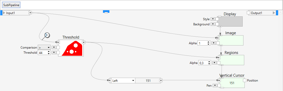
Calculating the left position.

Regions that have a left value of 0 (or <0) are regions touching (or crossing) the left border. This feature is sometimes used to filter out objects touching the left border.

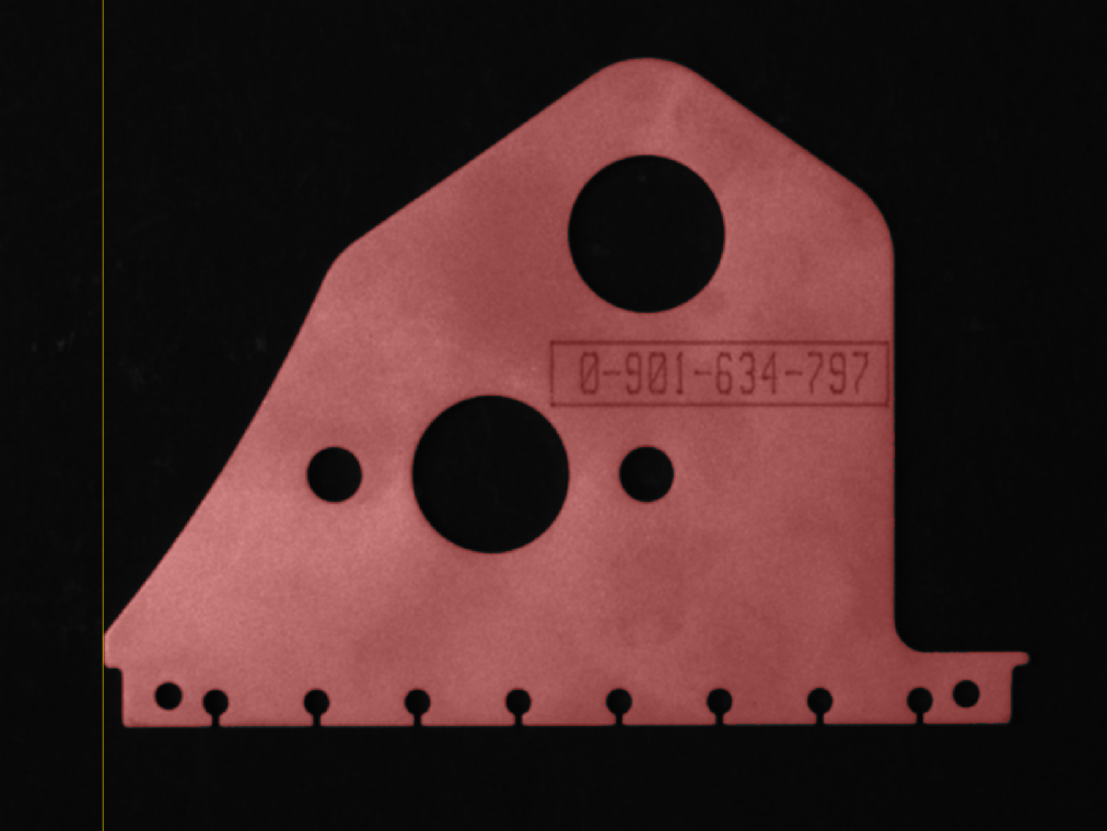
Visualizing the left position.

Since this is an integer coordinate, it is conceptually in the middle of the leftmost pixel.

Right

This calculates the maximal x coordinate (exclusive) of the region.

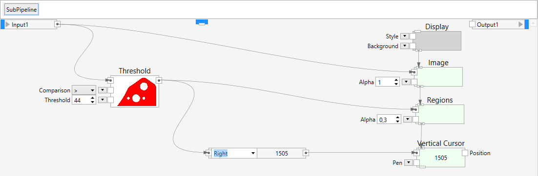
Calculating the right position.

Regions that have a right value equal to the image width (or bigger than the image width) are regions touching (or crossing) the right border. This feature is sometimes used to filter out objects touching the right border.

Visualizing the right position.

Since this is an integer coordinate, it is conceptually half a pixel right of the rightmost pixel.

Top

This calculates the minimal y coordinate (inclusive) of the region.

Calculating the top position.

Regions that have a top value of 0 (or <0) are regions touching (or crossing) the top border. This feature is sometimes used to filter out objects touching the top border.

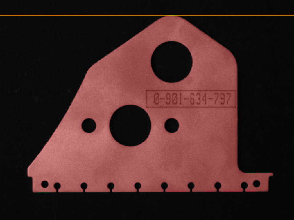
Visualizing the top position.

Since this is an integer coordinate, it is conceptually in the middle of the topmost pixel.

Bottom

This calculates the maximal y coordinate (exclusive) of the region.

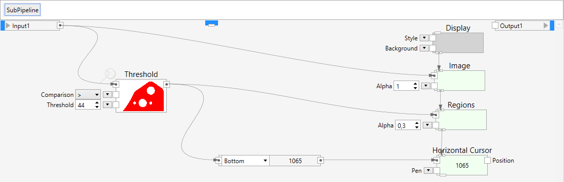
Calculating the left position.

Regions that have a bottom value equal to the image height (or bigger than the image height) are regions touching (or crossing) the bottom border. This feature is sometimes used to filter out objects touching the bottom border.

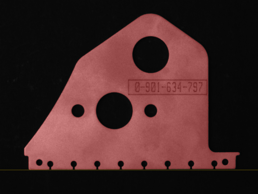
Visualizing the bottom position.

Since this is an integer coordinate, it is conceptually in the middle of the topmost pixel.

Width

This calculates the axis-parallel width of the region.

Calculating the width of an object.

Height

This calculates the axis-parallel height of the region.

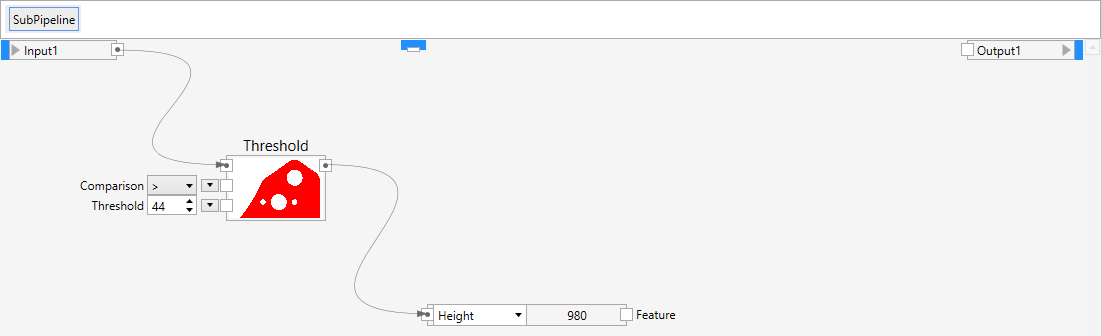
Calculating the height of an object.

Aspect Ratio

This calculates the axis-parallel aspect ratio of the region. The aspect ratio is calculated according to the following formula:

\[r=\frac{w}{h}\]

where w is the width and h is the height.

Calculating the aspect ratio of an object.

Sphericity

This calculates the sphericity of the region. The sphericity is defined as the quotient of the diameter of a circle having the same area as the object and the maximum feret diameter of the object. The sphericity is calculated according to the following formula:

\[s=\frac{2*sqrt{\frac{a}{pi}}}{f}\]

where a is the area and f is the maximum feret diameter.

Circularity

This calculates the circularity of the region. The circularity is defined as the quotient of the perimeter of a circle having the same area as the object and the perimeter of the object. The circularity is calculated according to the following formula:

\[c=\frac{2*sqrt{a*pi}}{p}\]

where a is the area and p is the perimeter.

Roundness

This calculates the roundness of the region. The roundness is defined as the quotient of the area of the object and the area of the minimum bounding circle. The roundness is calculated according to the following formula:

\[r=\frac{a}{c}\]

where a is the area and c is the area of the minimum bounding circle.

Roughness

This calculates the roughness of the region. The roughness is defined as the quotient of the perimeter of the object and the perimeter of the convex hull. The roughness is calculated according to the following formula:

\[r=\frac{p}{c}\]

where p is the perimeter and c is the perimeter of the convex hull.

Bounds

This calculates the bounds of the region.

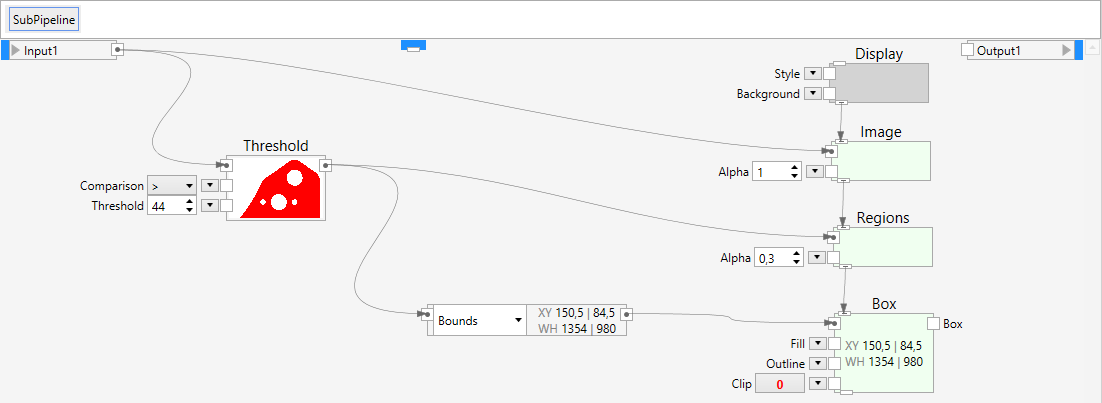
Calculating the bounds of an object.

The bounds are an axis parallel rectangle that encompasses the whole region tightly.

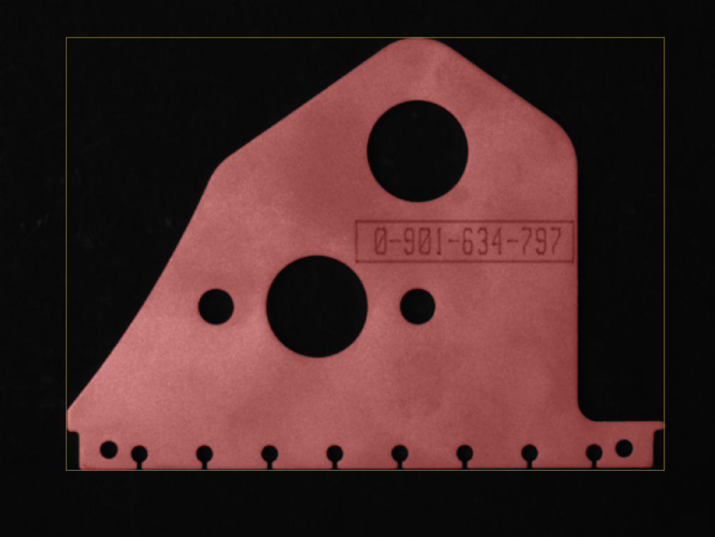
Visualizing the bounds.

Perimeter

The perimeter of a region specifies the length of the object outline.

Calculating the perimeter of an object.

Compactness

This calculates the compactness of the region.

Calculating the compactness of an object.

The compactness c is calculated from the region area a and the region perimeter p according to this formula:

\[c = \frac {p^{2}} {4 \pi a}\]

Convex Hull

This calculates a polyline that constitutes the convex hull of the region.

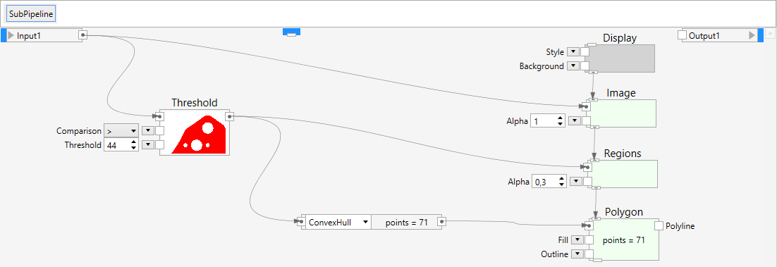
Calculating the convex hull of an object.

The convex hull encompasses the region tightly, like a rubberband.

Visualizing the convex hull.

The convex hull can be used to calculate further features, such as the area of the convex hull, the perimeter of the convex hull, as well as the minimum and maximum width of the convex hull. The minimum and the maximum width of the convex hull are calculated using a rotating caliper algorithm and are often called the Feret diameters.

Convex Area

This calculates the area enclosed by the convex hull.

Calculating the convex area of an object.

The convex area is always the same or bigger than the area of the original region. For the example image one can see right away that it is certainly bigger.

Perforation

This calculates the perforation of the region.

Calculating the perforation of an object.

The perforation p is calculated from the region area a and the area of the holes ah according to this formula:

\[p = \frac { { a }_{ h } }{ a }\]

The perforation is zero for a region that has no holes, and it increases the more holes the region has. The perforation is scale invariant.

Convexity

This calculates the convexity of the region.

Calculating the convexity of an object.

The convexity c is calculated from the region area a and the convex area ac according to this formula:

\[c = \frac { a }{ { a }_{ c } }\]

The convexity is 1 for a region that already is convex. It is smaller than 1 for non-convex regions. The convexity is scale invariant.

Convex Perimeter

This calculates the perimeter of the convex hull polygon.

Calculating the convex perimeter of an object.

Minimum Feret Diameter

This calculates the minimum feret diameter of the convex hull polygon. The minimum feret diameter is calculated using a rotating calipers algorithm.

Calculating the minimum feret diameter of an object.

Maximum Feret Diameter

This calculates the maximum feret diameter of the convex hull polygon. The maximum feret diameter is calculated using a rotating calipers algorithm.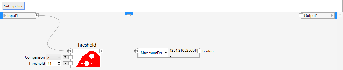

Minimum Bounding Circle

This calculates the smallest bounding circle of the region.

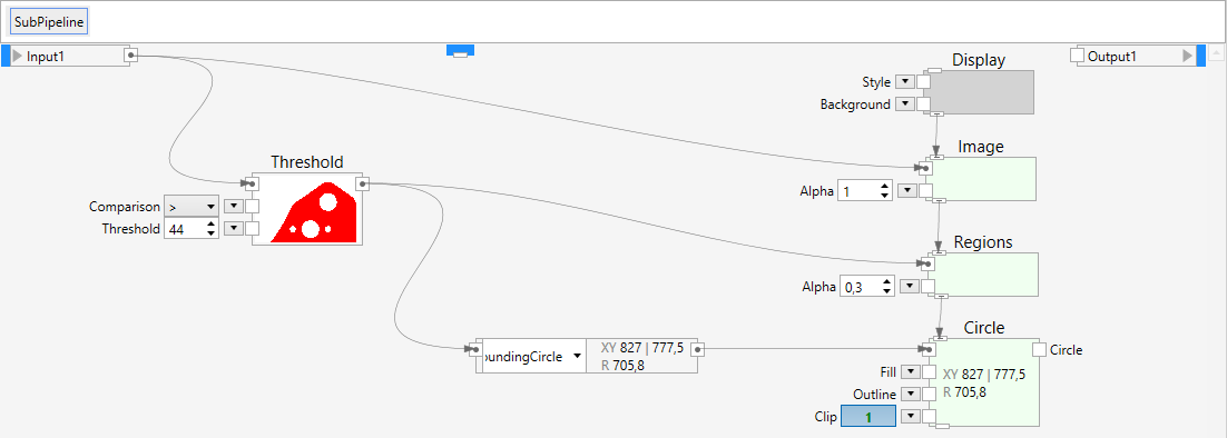
Calculating the minimum bounding circle of an object.

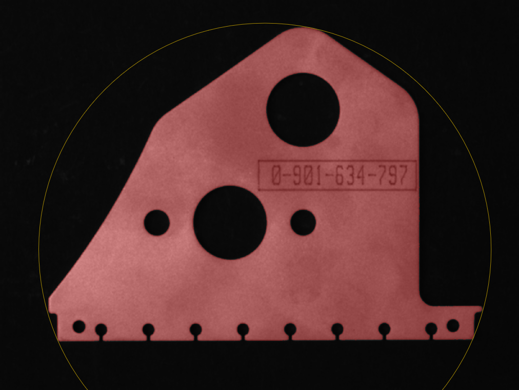
Visualizing the minimum bounding circle of an object.

Inner Contour Perimeter

This calculates the object perimeter using the inner contour. The inner contour is a counter-clockwise chain code of object boundary pixels. The inner contour exclusively lies on object pixels and is an 8-connected contour.

Calculating the inner contour perimeter of an object.

The inner contour is 8-connected. The contour length sums the contour segments for each of the chain code directions. Horizontal and vertical directions count as 1, diagonal directions count as \(\sqrt{2}\).

Outer Contour Perimeter

This calculates the object perimeter using the outer contour. The outer contour is a clockwise chain code of background pixels just outside the object. The outer contour exclusively lies on background pixels and is a 4-connected contour.

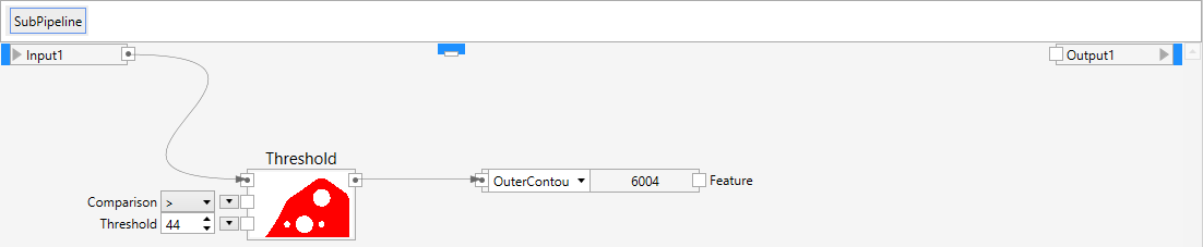
Calculating the outer contour perimeter of an object.

The outer contour is 4-connected. The contour length sums the contour segments for each of the chain code directions. Horizontal and vertical directions count as 1, diagonal directions are not used.

Region-based Moments

This calculates the region-based raw moments. There is a specific chapter about moments that you can consult, if you want to learn more about moments and how they are implemented. Here, in the context of blob analysis, they are documented only briefly.

Calculating the region based moments of an object.

The region-based raw moments are calculated up to the third order, according to the following formula:

\[M_{pq} = \sum _{xy} x^{p} y^{q}\]

The moments class has the properties m00, m10, m01, m20, m11, m02, m30, m21, m12 and m03 to read the respective moment.

Region-based Normalized Moments

This calculates the region-based normalized moments.

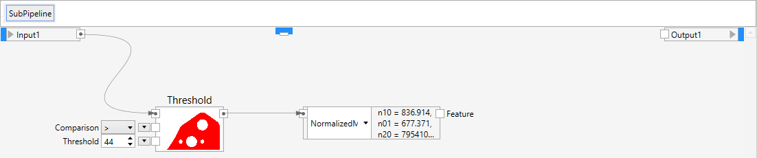
Calculating the region based normalized moments of an object.

They are calculated up to the third order, according to the following formula:

\[N_{pq}=\frac{M_{pq}}{M_{00}}\]

Normalized moments are invariant with respect to scaling, but are not invariant with respect to translation and rotation.

You can use the properties n10, n01, n20, n11, n02, n30, n21, n12 and n03 to read the respective normalized moments.

Region-based Centroid

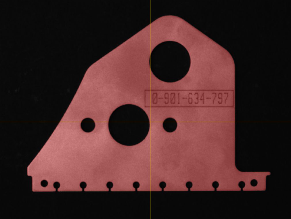
This calculates the region-based object centroid. The centroid is a property of the normalized moments.

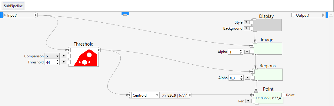
Calculating the region based centroid of an object.

The centroid is the center of gravity and calculated according to the following formula:

\[\begin{split}\bigl(\begin{matrix} x \\ y \end{matrix}\bigr) = \bigl(\begin{matrix} \frac { { N }_{ 10 } }{ { N }_{ 00 } } \\ \frac { { N }_{ 01 } }{ { N }_{ 00 } } \end{matrix}\bigr)\end{split}\]

Region-based Central Moments

This calculates the region-based central moments.

Calculating the region based central moments of an object.

They are calculated up to the third order according to the following formula:

\[\mu_{ pq }=\frac { 1 }{ M_{ 00 } } \sum _{ x }^{ }{ \sum _{ y }^{ }{ { (x-\overline { x } ) }^{ p }{ (y-\overline { y } ) }^{ q } } }\]

Central moments are invariant with respect to translation, but are not invariant with respect to rotation. You can use the properties mu20, mu11, mu02, mu30, mu21, mu12 and mu03 to read the respective central moments.

Region-based Equivalent Ellipse

This calculates the region_based equivalent ellipse of the object. The equivalent ellipse is built by combining properties from the normalized and the central moments.

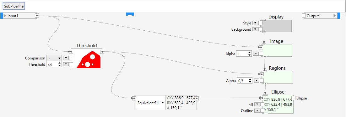
Calculating the region based equivalent ellipse of an object.

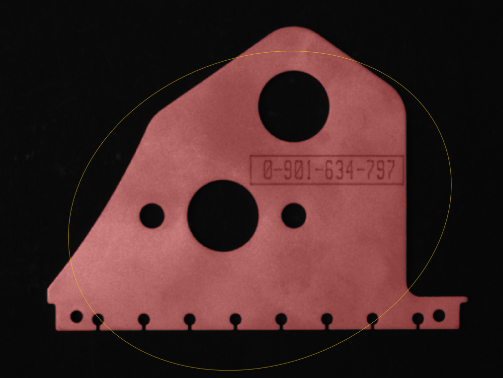
Visualizing the region based equivalent ellipse of an object.

Region-based Scale Invariant Moments

This calculates the region-based scale-invariant moments.

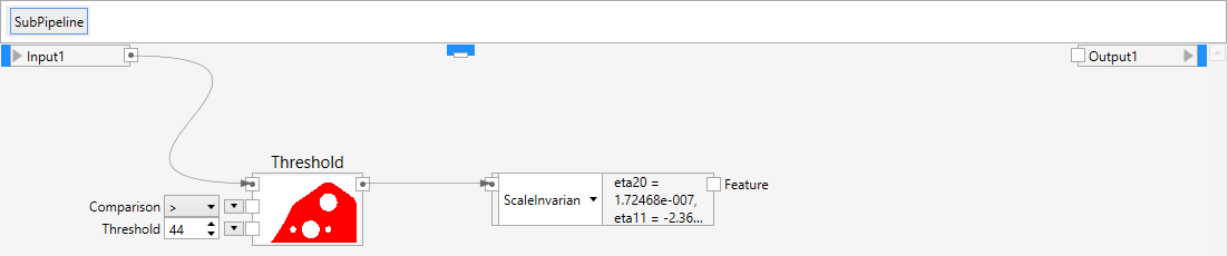
Calculating the region based scale invariant moments of an object.

They are calculated up to the third order according to the following formula:

\[\eta_{pq}={\frac{\mu_{pq}}{\mu_{00}^{\frac{p+q}{2}+1}}}\]

Scale-invariant moments are invariant with respect to translation and scaling, but are not invariant with respect to rotation.

You can use the properties eta20, eta11, eta02, eta30, eta21, eta12 and eta03 to read the respective scale invariant moments.

Region-based Hu Moments

This calculates the region-based Hu moments. The formulas are described in the chapter about moments.

Calculating the region based Hu moments of an object.

Hu’s moments are invariant with respect to translation, scaling and rotation.

The formulas for Hu’s moments are:

\[\begin{split}\begin{aligned} {\phi}_{{1}} & = & {{\eta}_{{20}}+{\eta}_{{02}}} \\ {\phi}_{{2}} & = & {({\eta}_{{20}}-{\eta}_{{02}})^2+4{\eta}_{{11}}^2} \\ {\phi}_{{2}} & = & {({\eta}_{{20}}-{\eta}_{{02}})^2+4{\eta}_{{11}}^2} \\ {\phi}_{{4}} & = & {({\eta}_{{30}}+{\eta}_{{12}})^2+({\eta}_{{21}}+{\eta}_{{03}})^2} \\ {\phi}_{{5}} & = & {({\eta}_{{30}}-3{\eta}_{{12}})({\eta}_{{30}}+{\eta}_{{12}})\left[({\eta}_{{30}}+{\eta}_{{12}})^2-3({\eta}_{{21}}+{\eta}_{{03}})^2\right]} \nonumber \\ & & {}{+(3{\eta}_{{21}}-{\eta}_{{03}})({\eta}_{{21}}+{\eta}_{{03}})\left[3({\eta}_{{30}}+{\eta}_{{12}})^2-({\eta}_{{21}}+{\eta}_{{03}})^2\right]} \\ {\phi}_{{6}} & = & {({\eta}_{{20}}-{\eta}_{{02}})\left[({\eta}_{{30}}+{\eta}_{{12}})^2-({\eta}_{{21}}+{\eta}_{{03}})^2\right]} \nonumber \\ & & {}{+4{\eta}_{{11}}({\eta}_{{30}}+{\eta}_{{12}})({\eta}_{{21}}+{\eta}_{{03}})} \\ {\phi}_{{7}} & = & {(3{\eta}_{{21}}-3{\eta}_{{03}})({\eta}_{{30}}+{\eta}_{{12}})\left[({\eta}_{{30}}+{\eta}_{{12}})^2-3({\eta}_{{21}}+{\eta}_{{03}})^2\right]} \nonumber \\ & & {}{-({\eta}_{{30}}-3{\eta}_{{12}})({\eta}_{{21}}+{\eta}_{{03}})\left[3({\eta}_{{30}}+{\eta}_{{12}})^2-({\eta}_{{21}}+{\eta}_{{03}})^2\right]}\end{aligned}\end{split}\]

You can use the properties phi1, phi2, phi3, phi4, phi5, phi6 and phi7 to read the respective Hu moment.

Region-based Flusser Moments

This calculates the region-based Flusser moments. The formulas are described in the chapter about moments.

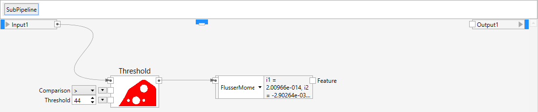
Calculating the region based Flusser moments of an object.

Flusser’s moments are invariant with respect to affine transformations.

The formulas for Flusser’s moments are:

\[\begin{split}\begin{aligned} {I}_{{1}} & = & {\frac{{\mu}_{{20}}{\mu}_{{02}}-{\mu}_{{11}}^2}{{\mu}_{{00}}^4}} \\ {I}_{{2}} & = & {\frac{{\mu}_{{30}}^2{\mu}_{{03}}^2-6{\mu}_{{30}}{\mu}_{{21}}{\mu}_{{12}}{\mu}_{{03}}+4{\mu}_{{30}}{\mu}_{{12}}^3+4{\mu}_{{21}}^3{\mu}_{{03}}-3{\mu}_{{21}}^2{\mu}_{{12}}^2}{{\mu}_{{00}}^10}} \\ {I}_{{3}} & = & {\frac{{\mu}_{{20}}({\mu}_{{21}}{\mu}_{{03}}-{\mu}_{{12}}^2)-{\mu}_{{11}}({\mu}_{{30}}{\mu}_{{03}}-{\mu}_{{21}}{\mu}_{{12}}))}{{\mu}_{{00}}^7}} \nonumber \\ & & {+\frac{{\mu}_{{02}}({\mu}_{{30}}{\mu}_{{12}}-{\mu}_{{21}}^2)}{{\mu}_{{00}}^7}} \\ {I}_{{4}} & = & {\frac{{\mu}_{{20}}^3{\mu}_{{03}}^2-6{\mu}_{{20}}^2{\mu}_{{11}}{\mu}_{{12}}({\mu}_{{03}}-6{\mu}_{{20}}^2{\mu}_{{02}}{\mu}_{{21}}){\mu}_{{03}}}{{\mu}_{{00}}^{11}}} \nonumber \\ & & {+\frac{9{\mu}_{{20}}^2{\mu}_{{02}}{\mu}_{{12}}^2+12{\mu}_{{20}}{\mu}_{{11}}^2{\mu}_{{21}}{\mu}_{{03}}+6{\mu}_{{20}}{\mu}_{{11}}{\mu}_{{02}}{\mu}_{{30}}{\mu}_{{03}}}{{\mu}_{{00}}^{11}}} \nonumber \\ & & {-\frac{18{\mu}_{{20}}{\mu}_{{11}}{\mu}_{{02}}{\mu}_{{21}}{\mu}_{{12}}+8{\mu}_{{11}}^3{\mu}_{{30}}{\mu}_{{03}}+6{\mu}_{{20}}{\mu}_{{02}}^2{\mu}_{{30}}{\mu}_{{12}}}{{\mu}_{{00}}^{11}}} \nonumber \\ & & {+\frac{9{\mu}_{{20}}{\mu}_{{02}}^2{\mu}_{{21}}^2+12{\mu}_{{11}}^2{\mu}_{{02}}{\mu}_{{30}}{\mu}_{{12}}-6{\mu}_{{11}}{\mu}_{{02}}^2{\mu}_{{30}}{\mu}_{{21}}}{{\mu}_{{00}}^{11}}} \nonumber \\ & & {+\frac{{\mu}_{{02}}^3{\mu}_{{30}}^2}{{\mu}_{{00}}^{11}}}\end{aligned}\end{split}\]

You can use the properties i1, i2, i3, and i4 to read the respective flusser moments.

Number of Holes

This calculates the number of holes of the region.

Calculating the number of holes of an object.

Area of Holes

This calculates the total area of the holes of the region.

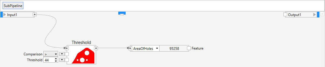
Calculating the area of all holes of an object.

Fiber Length

This calculates an approximation of a fiber length. This measurement is only valid for elongated objects. The fiber length is approximated as half the perimeter.

Fiber Width

This calculates an approximation of a fiber width. The fiber width is approximated as twice the maximum value of the distance transform.

Bounding Rectangle

This calculates a bounding rectangle of the region.

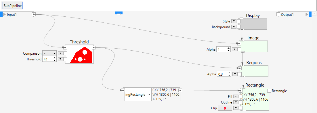
Calculating the bounding rectangle of an object.

The rectangle has the same orientation as the equivalent ellipse.

Minimum Area Bounding Rectangle

This calculates a bounding rectangle of the region with a minimal area.

Calculating the bounding rectangle of an object.

The result is the rectangle with the smallest area bounding the region.

Visualizing the bounding rectangle of an object.

Minimum Perimeter Bounding Rectangle

This calculates a bounding rectangle of the region with a minimal perimeter.

Calculating the bounding rectangle of an object.

The result is the rectangle with the smallest perimeter bounding the region.

Visualizing the bounding rectangle of an object.

Pixel Based Features

In contrast to region-based features, pixel-based features use the pixel values in addition to the region definition. Pixel-based features are necessary since some features, such as the minimum pixel value, cannot be calculated given the region alone. However, the calculation of pixel-based features is slower than the calculation of region-based features.

Minimum Position

This calculates the minimum position value.

blob_features b(gray.get_view(), objects[0]);
point_3d<int> minimum = *b.get_minimum_position();

When calculating the minimum position for color images, the color is treated as a vector and the minimum is determined by comparing the Euclidean vector length.

Minimum

This calculates the minimum value.

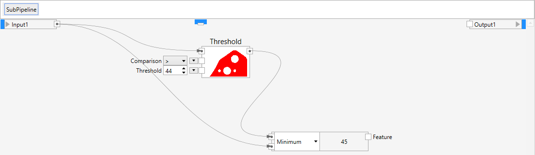
Calculating the minimum value of an object.

When calculating the minimum for color images, the color is treated as a vector and the minimum is determined by comparing the Euclidean vector length.

Maximum Position

This calculates the maximum position value.

blob_features b(gray.get_view(), objects[0]);
point_3d<int> maximum = *b.get_maximum_position();

When calculating the minimum position for color images, the color is treated as a vector and the minimum is determined by comparing the Euclidean vector length.

Maximum

This calculates the maximum value.

Calculating the maximum value of an object.

When calculating the maximum for color images, the color is treated as a vector and the maximum is determined by comparing the Euclidean vector length.

Total

This calculates the total value.

Calculating the total value of an object.

The total is the sum of all pixel values of the object:

\[T=\sum I\]

Mean

This calculates the mean value.

Calculating the mean value of an object.

The mean is calculated according to the following formula:

\[M = \frac { T }{ n }\]

where T is the total value and n is the number of pixels (i.e. the area) of the blob.

Standard Deviation

This calculates the standard deviation value. Standard deviation is a measure of how wide the distribution of values is.

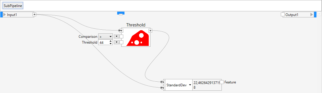
Calculating the standard deviation of an object.

The standard deviation is calculated according to the following formula:

\[\sigma = \sqrt {\frac { 1 }{ n } \sum {}{(I-E)^2}}\]

Skewness

This calculates the skewness value. Skewness can be understood as a measure of asymmetry in the distribution, i.e. how much it deviates from a gauss-shaped curve.

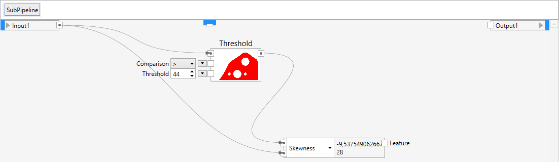
Calculating the skewness of an object.

The skewness is calculated according to the following formula:

\[\sigma = \sqrt[3]{\frac { 1 }{ n } \sum {}{(I-E)^3}}\]

Contrast

This calculates the channel-wise contrast.

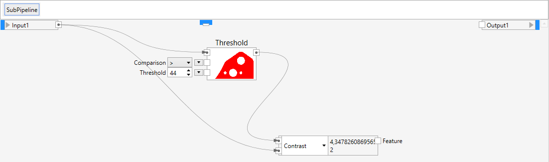
Calculating the contrast of an object.

The contrast is calculated according to the following formula:

\[c=\frac {max}{min + 1}\]

Weber Contrast

This calculates the channel-wise contrast acoording to Weber’s formula.

Calculating the contrast of an object.

The contrast is calculated according to the following formula:

\[c=\frac {max - min}{min + 1}\]

Michelson Contrast

This calculates the channel-wise contrast acoording to Michelson’s formula.

Calculating the contrast of an object.

The contrast is calculated according to the following formula:

\[c=\frac {max - min}{max + min + 1}\]

Pixel-based Moments

This calculates the pixel-based raw moments. There is a specific chapter about moments that you can consult, if you want to learn more about moments and how they are implemented. Here, in the context of blob analysis, they are documented only briefly.

Calculating the pixel based moments of an object.

The pixel-based raw moments are calculated up to the third order, according to the following formula:

\[M_{pq} = \sum _{xy} x^{p} y^{q} I_{xy}\]

Pixel based moments are similar to region-based moments, but they make use of pixel values in addition. The brighter a pixel is the more weight it has in the calculation of the moment.

If color images are used, they are converted to monochrome, before the respective pixel-based moment is calculated. The moments class has the properties m00, m10, m01, m20, m11, m02, m30, m21, m12 and m03 to read the respective moment.

Pixel-based Normalized Moments

This calculates the pixel-based normalized moments.

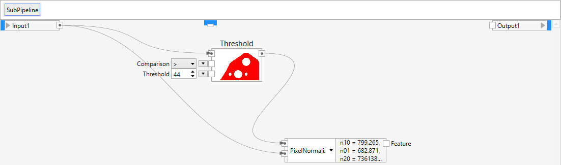
Calculating the pixel based normalized moments of an object.

They are calculated up to the third order, according to the following formula:

\[N_{pq}=\frac{M_{pq}}{M_{00}}\]

Pixel based moments are similar to region-based moments, but they use pixel values in addition. The brighter a pixel is the more weight it has in the calculation of the moment.

If color images are used, they are converted to monochrome, before the respective pixel-based moment is calculated. You can use the properties n10, n01, n20, n11, n02, n30, n21, n12 and n03 to read the respective normalized moments.

Pixel-based Centroid

This calculates the pixel-based object centroid. The centroid is a property of the normalized moments.

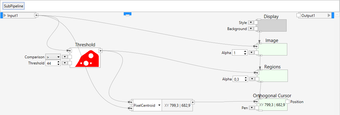
Calculating the pixel based centroid of an object.

The centroid is the center of gravity and calculated according to the following formula:

\[\begin{split}\left( \begin{matrix} x \\ y \end{matrix} \right) =\left( \begin{matrix} \frac { { N }_{ 10 } }{ { N }_{ 00 } } \\ \frac { { N }_{ 01 } }{ { N }_{ 00 } } \end{matrix} \right)\end{split}\]

Visualizing the pixel based centroid of an object.

Pixel based centroids are similar to region-based centroids, but they use pixel values in addition. The brighter a pixel is the more weight it has in the calculation of the moment.

If color images are used, they are converted to monochrome, before the respective pixel-based moment is calculated.

Pixel-based Central Moments

This calculates the pixel-based central moments.

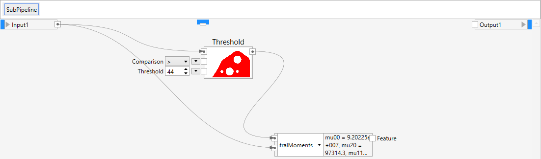
Calculating the pixel based central moments of an object.

They are calculated up to the third order according to the following formula:

\[\mu_{pq}=\frac { 1 }{ M_{ 00 } } \sum _{ x }^{ }{ \sum _{ y }^{ }{ { (x-\overline { x } ) }^{ p }{ (y-\overline { y } ) }^{ q }{ I }_{ xy } } }\]

Central moments are invariant with respect to translation, but are not invariant with respect to rotation. Pixel based moments are similar to region-based moments, but they use pixel values in addition. The brighter a pixel is the more weight it has in the calculation of the moment.

If color images are used, they are converted to monochrome, before the respective pixel-based moment is calculated. You can use the properties mu20, mu11, mu02, mu30, mu21, mu12 and mu03 to read the respective central moments.

Pixel-based Equivalent Ellipse

This calculates the pixel-based equivalent ellipse of the object. The equivalent ellipse is built by combining properties from the normalized and the central moments.

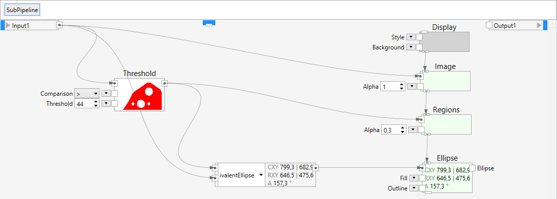
Calculating the pixel based equivalent ellipse of an object.

Pixel based equivalent ellipses are similar to region-based equivalent ellipses, but they use pixel values in addition. The brighter a pixel is the more weight it has in the calculation of the moment.

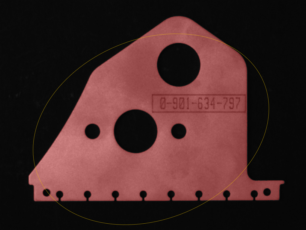
Visualizing the pixel based equivalent ellipse of an object.

If color images are used, they are converted to monochrome, before the respective pixel-based moment is calculated.

Pixel-based Scale Invariant Moments

This calculates the pixel-based scale-invariant moments.

Calculating the pixel based scale invariant moments of an object.

They are calculated up to the third order, according to the following formula:

\[\eta_{pq}={\frac{\mu_{pq}}{\mu_{00}^{\frac{p+q}{2}+1}}}\]

Scale-invariant moments are invariant with respect to translation and scaling, but are not invariant with respect to rotation.

Pixel based moments are similar to region-based moments, but they use pixel values in addition. The brighter a pixel is the more weight it has in the calculation of the moment.

If color images are used, they are converted to monochrome, before the respective pixel-based moment is calculated. You can use the properties eta20, eta11, eta02, eta30, eta21, eta12 and eta03 to read the respective scale invariant moments.

Pixel-based Hu Moments

This calculates the pixel-based Hu moments.

Calculating the pixel based Hu of an object.

The formulas for Hu’s moments are:

\[\begin{split}\begin{aligned} {\phi}_{{1}} & = & {{\eta}_{{20}}+{\eta}_{{02}}} \\ {\phi}_{{2}} & = & {({\eta}_{{20}}-{\eta}_{{02}})^2+4{\eta}_{{11}}^2} \\ {\phi}_{{3}} & = & {({\eta}_{{30}}-3{\eta}_{{12}})^2+(3{\eta}_{{21}}-{\eta}_{{03}})^2} \\ {\phi}_{{4}} & = & {({\eta}_{{30}}+{\eta}_{{12}})^2+({\eta}_{{21}}+{\eta}_{{03}})^2} \\ {\phi}_{{5}} & = & {({\eta}_{{30}}-3{\eta}_{{12}})({\eta}_{{30}}+{\eta}_{{12}})\left[({\eta}_{{30}}+{\eta}_{{12}})^2-3({\eta}_{{21}}+{\eta}_{{03}})^2\right]} \nonumber \\ & & {}{+(3{\eta}_{{21}}-{\eta}_{{03}})({\eta}_{{21}}+{\eta}_{{03}})\left[3({\eta}_{{30}}+{\eta}_{{12}})^2-({\eta}_{{21}}+{\eta}_{{03}})^2\right]} \\ {\phi}_{{6}} & = & {({\eta}_{{20}}-{\eta}_{{02}})\left[({\eta}_{{30}}+{\eta}_{{12}})^2-({\eta}_{{21}}+{\eta}_{{03}})^2\right]} \nonumber \\ & & {}{+4{\eta}_{{11}}({\eta}_{{30}}+{\eta}_{{12}})({\eta}_{{21}}+{\eta}_{{03}})} \\ {\phi}_{{7}} & = & {(3{\eta}_{{21}}-3{\eta}_{{03}})({\eta}_{{30}}+{\eta}_{{12}})\left[({\eta}_{{30}}+{\eta}_{{12}})^2-3({\eta}_{{21}}+{\eta}_{{03}})^2\right]} \nonumber \\ & & {}{-({\eta}_{{30}}-3{\eta}_{{12}})({\eta}_{{21}}+{\eta}_{{03}})\left[3({\eta}_{{30}}+{\eta}_{{12}})^2-({\eta}_{{21}}+{\eta}_{{03}})^2\right]}\end{aligned}\end{split}\]

Hu’s moments are invariant with respect to translation, scaling and rotation.

Pixel based moments are similar to region-based moments, but they use pixel values in addition. The brighter a pixel is the more weight it has in the calculation of the moment.

If color images are used, they are converted to monochrome, before the respective pixel-based moment is calculated. You can use the properties phi1, phi2, phi3, phi4, phi5, phi6 and phi7 to read the respective Hu moment.

Pixel-based Flusser Moments

This calculates the pixel-based Flusser moments.

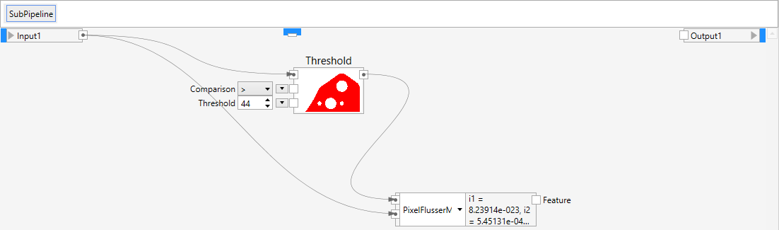
Calculating the pixel based Flusser moments of an object.

The formulas for Flusser’s moments are:

\[\begin{split}\begin{aligned} {I}_{{1}} & = & {\frac{{\mu}_{{20}}{\mu}_{{02}}-{\mu}_{{11}}^2}{{\mu}_{{00}}^4}} \\ {I}_{{2}} & = & {\frac{{\mu}_{{30}}^2{\mu}_{{03}}^2-6{\mu}_{{30}}{\mu}_{{21}}{\mu}_{{12}}{\mu}_{{03}}+4{\mu}_{{30}}{\mu}_{{12}}^3+4{\mu}_{{21}}^3{\mu}_{{03}}-3{\mu}_{{21}}^2{\mu}_{{12}}^2}{{\mu}_{{00}}^10}} \\ {I}_{{3}} & = & {\frac{{\mu}_{{20}}({\mu}_{{21}}{\mu}_{{03}}-{\mu}_{{12}}^2)-{\mu}_{{11}}({\mu}_{{30}}{\mu}_{{03}}-{\mu}_{{21}}{\mu}_{{12}}))}{{\mu}_{{00}}^7}} \nonumber \\ & & {+\frac{{\mu}_{{02}}({\mu}_{{30}}{\mu}_{{12}}-{\mu}_{{21}}^2)}{{\mu}_{{00}}^7}} \\ {I}_{{4}} & = & {\frac{{\mu}_{{20}}^3{\mu}_{{03}}^2-6{\mu}_{{20}}^2{\mu}_{{11}}{\mu}_{{12}}({\mu}_{{03}}-6{\mu}_{{20}}^2{\mu}_{{02}}{\mu}_{{21}}){\mu}_{{03}}}{{\mu}_{{00}}^{11}}} \nonumber \\ & & {+\frac{9{\mu}_{{20}}^2{\mu}_{{02}}{\mu}_{{12}}^2+12{\mu}_{{20}}{\mu}_{{11}}^2{\mu}_{{21}}{\mu}_{{03}}+6{\mu}_{{20}}{\mu}_{{11}}{\mu}_{{02}}{\mu}_{{30}}{\mu}_{{03}}}{{\mu}_{{00}}^{11}}} \nonumber \\ & & {-\frac{18{\mu}_{{20}}{\mu}_{{11}}{\mu}_{{02}}{\mu}_{{21}}{\mu}_{{12}}+8{\mu}_{{11}}^3{\mu}_{{30}}{\mu}_{{03}}+6{\mu}_{{20}}{\mu}_{{02}}^2{\mu}_{{30}}{\mu}_{{12}}}{{\mu}_{{00}}^{11}}} \nonumber \\ & & {+\frac{9{\mu}_{{20}}{\mu}_{{02}}^2{\mu}_{{21}}^2+12{\mu}_{{11}}^2{\mu}_{{02}}{\mu}_{{30}}{\mu}_{{12}}-6{\mu}_{{11}}{\mu}_{{02}}^2{\mu}_{{30}}{\mu}_{{21}}}{{\mu}_{{00}}^{11}}} \nonumber \\ & & {+\frac{{\mu}_{{02}}^3{\mu}_{{30}}^2}{{\mu}_{{00}}^{11}}}\end{aligned}\end{split}\]

Flusser’s moments are invariant with respect to affine transformations.

Pixel based moments are similar to region-based moments, but they use pixel values in addition. The brighter a pixel is the more weight it has in the calculation of the moment.

If color images are used, they are converted to monochrome, before the respective pixel-based moment is calculated. You can use the properties i1, i2, i3, and i4 to read the respective usser moments.

Object Filtering

Filtering is the process of removing objects that satisfy a certain condition. Examples of filtering are removal of small objects caused by noise, or removal of objects touching the image border, because these objects would be partial anyway and their features would be wrong.

Here is an example that removes objects with an area smaller than 100 pixels:

Removing small objects.

Here is another example that removes objects which are touching the left border:

Removing objects near left boundary.

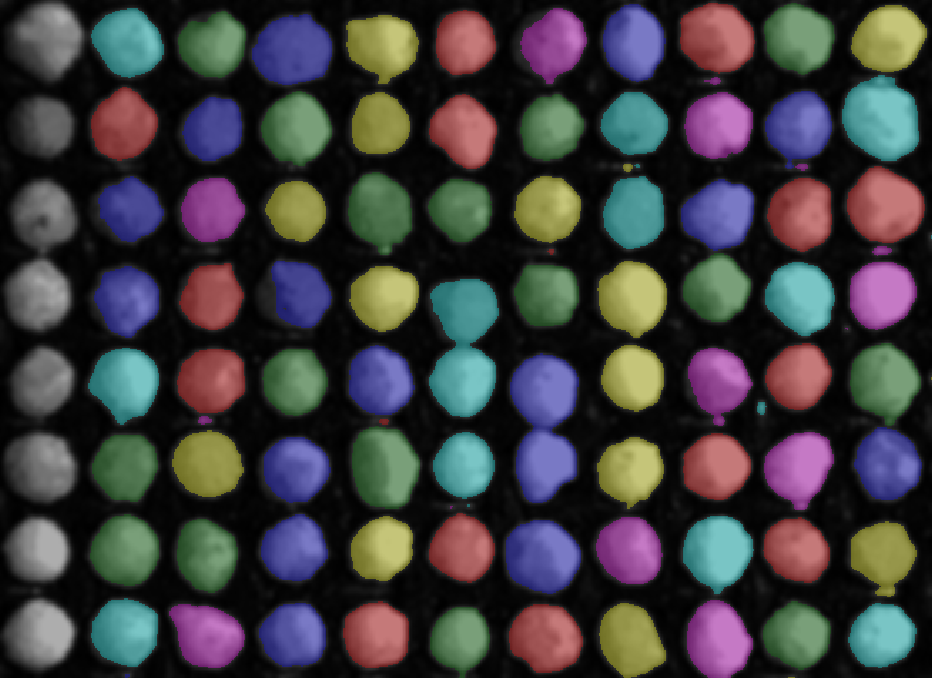
Objects near left border have been removed..

Filters can be chained in order to create more complex conditions.