Dataflow

nVision can be programmed graphically using the concept of a dataflow pipeline.

While the user is executing image processing commands, nVision builds a pipeline of those commands. Such a pipeline is essentially a program that can then be executed over and over again, for potentially many images. The image data flows through the pipeline much like water flows through a system of pipes.

Here is an example of such a pipeline, where the data flows from top to bottom.

A linear pipeline, where the data flows from top to bottom, following the arrows.

It is particularly easy to create this pipeline, just by issuing the following commands, one after the other:

	Command	Description
	File - Open	Opens a file (cells.tif from samples).
	Segmentation - Threshold	Binary thresholding (> 100).
	Segmentation - Connected Components	Split into connected components.
	Segmentation - Blob Analysis	Calculate features for objects.

There are some parameters on top of some pipeline steps that can be changed and that affect the outcome of the pipeline. If you want to know what these parameters are, move the mouse on top of the parameters editor and look at the tooltip that appears. Whenever a parameter is changed by the user, the pipeline reruns and the results are re-calculated.

What you have built this way is a linear sequence of steps - or pipeline nodes - and this is essentially a very simple program.

Linear Pipeline

A linear pipeline is the easiest way to create a program in nVision.

A linear pipeline is displayed at the left of the workbench. Each image can have its own pipeline and the pipeline is tightly coupled with the image. When an image is saved, the pipeline is saved along the image under the same name but with .xpipe added. If you save an image under the name image.tif, the associated pipeline will be save at the same location under the name image.tif.xpipe.

A pipeline can be explicitely exported to a file, in case you want to reuse it for a different image. This is done with the Export Pipeline command from the File menu. To actually re-use a pipeline for a different image, use the Import Pipeline command from the File menu.

A pipeline can also be used for a batch of files in a folder. In this case, you would first load the set of file using the Open Folder command from the File menu, and then load a pipeline using the Import Pipeline command from the File menu. On the Pipeline menu are commands that can then be used to run the pipeline on all images, or to single step forward or backward through the sequence of files.

The steps of a linear pipeline are called pipeline nodes or simply nodes.

A node in the linear pipeline. Data flows in from the top and out at the bottom. Parameters can be changed by the user using the controls at the top of the node. Output data is previewed in a little thumbnail presentation in the node.

Behind the scenes, building a linear pipeline is a complex process. When a command is executed from the menu, the associated node is appended to the existing pipeline. At the same time, it is connected to the pipeline, so that the data can flow to the new end. Also, the visualization in the workbench is changed, so that the result of the last pipeline node is shown.

The data that can flow through the pipeline is not restricted to images only. There are many more types of data, such as histograms, profiles, regions, blob analysis results or even numbers. Commands however may make sense for a limited set of types only. An image filter needs an image on input. As a consequence, when a linear pipeline is built, some commands on the menu may be grayed out, if the result of executing them would be an inconsistent linear pipeline.

Usually, the last node in a linear pipeline is selected, and new nodes are appended at the end. However, you can also select a node in the middle of the pipeline. In this case, a node would be inserted after the selected node. In such cases even more commands may be grayed out, since not only the input to the node must fit the available type, but also the output of the node.

Another feature of the linear pipeline are the previews that are displayed within the nodes. We have tried to make these previews as helpful as possible, so that it is easy for you to understand how a specific pipeline works. The previews are live, which you will appreciate if you have a camera connected.

Finally, the nodes in the linear pipeline have a context menu, which is shown when you move the mouse on top of the node:

	Command
	Show the node result in the workbench window.
	Toggle acquisition from a camera.

We encourage you to play with the commands and build pipelines as you wish. nVision is made to be explored by the user and we have tried to make this exploration phase as easy as possible. Once you know a few basics, nVision is very learnable, and a lot of its features can be found out by simple exploration, without the need of reading a lengthy manual.

Sub-Pipeline

Surprisingly many applications can be carried out using a linear pipeline, but at some time sooner or later, you will hit a task that cannot be solved this way. For this reason, we have created the possibility to work with branched pipelines. A branched pipeline can have multiple branches and is much more powerful and flexible than its linear variant. Here is an example of a very simple branched pipeline:

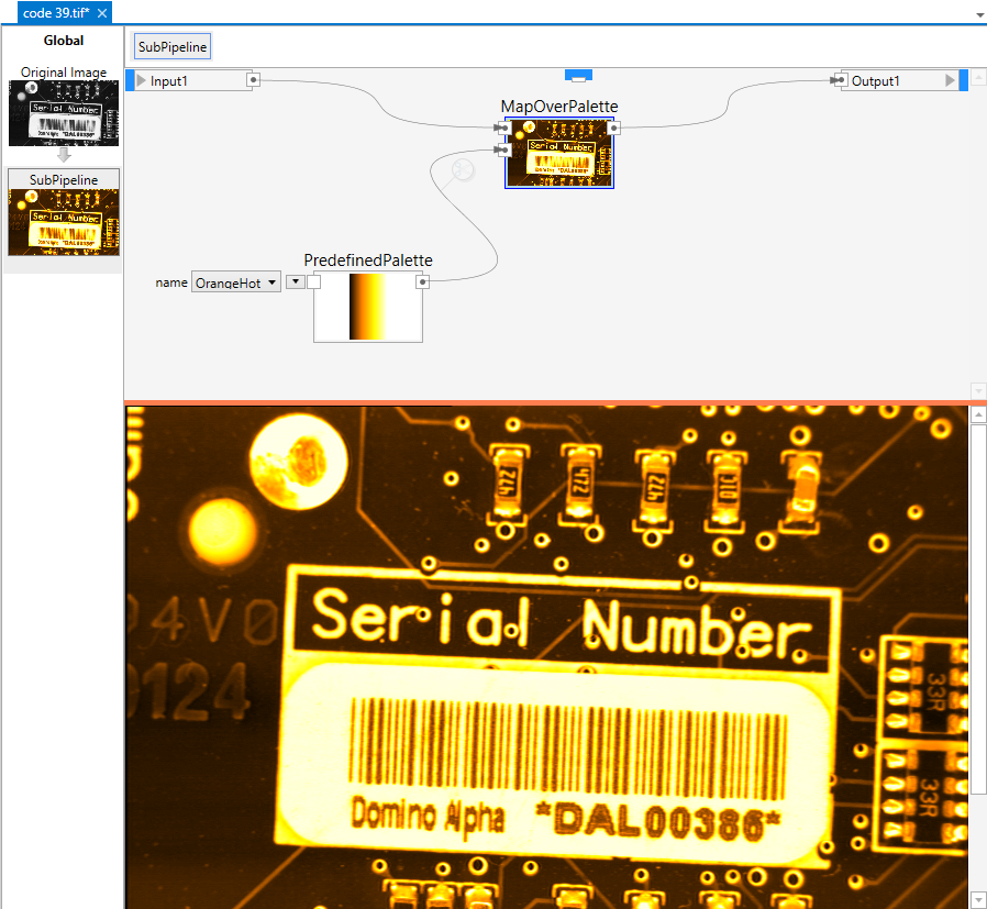
A very simple branched pipeline. It takes an image on its single input, maps it over a palette and outputs the result. Another node creates the palette by choosing between a set of predefined entries. Below the pipeline you see the result, which in this case is a colored image.

The ingredients of a branched pipeline are essentially the same as for the linear pipeline: nodes and connections between the nodes. With the increased flexibility comes a little bit more work for the user: the connections are no longer automatic, but must be done manually.

A node in the branched pipeline. Data flows in from the left and out at the right. Parameters can be changed by the user using the controls at the left of the node. Output data is previewed in a little thumbnail presentation in the node.

Although they are displayed slightly different, nodes in the linear and in the branched pipeline are equivalent. You can also see that the distinction between input and parameters is somewhat arbitrary. In fact, parameters are just additional inputs.

Inputs are either mandatory or optional. Mandatory inputs need to be connected to some other node upstream, otherwise the node will not be able to execute. If a node does cannot execute, it either displays a standard icon or nothing at all in its preview area. Optional inputs do not need to be connected and they show a little control element that allows to input a value. However, they can be connected to some other node upstream, and in this case the control element is hidden and the data is taken from the upstream node.

A sub-pipeline is created by executing the Subpipeline command from the Pipeline menu. This adds a sub-pipeline node to the linear pipeline. Since the sub-pipeline is empty at this time, the workbench shows an empty window, but at the top you see a tab with the name SubPipeline and an orange splitter. The splitter can be dragged down with the mouse, and if you do so, the upper portion of the window will display the branched pipeline area and the lower portion of the window will display the result. Since at this time the subpipeline is still empty, both areas will be mostly empty as well. In order to change the name of the sub-pipeline, click its title on top of the preview.

In the sub-pipeline, the commands are available via a context menu, which you can access by clicking with the right mouse button into the editor area. There are more commands available as in the linear case.

The context menu of the sub-pipeline.

The commands in the context menu are organized in groups. Most commands add a node to the pipeline editor canvas, which you can then drag around with the mouse by clicking somewhere inside its box. You can also connect the ports of the nodes to other ports in order to define the flow of data. Arrows can only be drawn between compatible ports, and icons guide you and help you to determine which ports are compatible.

At the top is a search box where you can type your command. For example, if you search a command related to histograms, just start typing hi, and the menu show only thos commands that contain the letter hi in their name (or group).

It is helpful to have the help window open while you learn programming. When you browse the menu, the help window will show help for the command you are browsing.

The Pipeline group contains a few commands that are related to pipeline handling. The Imaging group contains commands that are related to image processing. The Vision group contains commands related to particle analysis, gauging, template matching, barcode and matrixcode reading as well as OCR. The Graphics group contains commands to create graphical overlays and editors, and the Support group contains any other commands that support you in creating efficient pipelines.