Getting Started
The screen shot shows the various parts of the nVision application.

The various parts of the nVision application.
At the top there is a ribbon with commands to control the application.
At the bottom, there is the work area, consisting of the browser and the workbench, where the main interaction takes place.
Before we explain nVision in detail, let us show a few simple examples of how to work with nVision.
Particle Analysis
Let us assume that the current task is to count and measure particles.
1. Open the image
The first step is to load an image. nVision can acquire images from digital cameras, but for now let us load an image from disk, by using the File - Open command:

Load an image from disk.
In the dialog that opens, select the cells.tif file. The file is loaded and displayed both in the browser and in the work area.

nVision with a loaded image.
2. Segment the image
Segmenting the image is next. The particles - in this case the cell nuclei - should be separated from the background. This can be done with the Threshold command from the ribbon’s Segmentation tab.

Segmenting an image with the threshold command.
A threshold of 100 works nicely for this image.
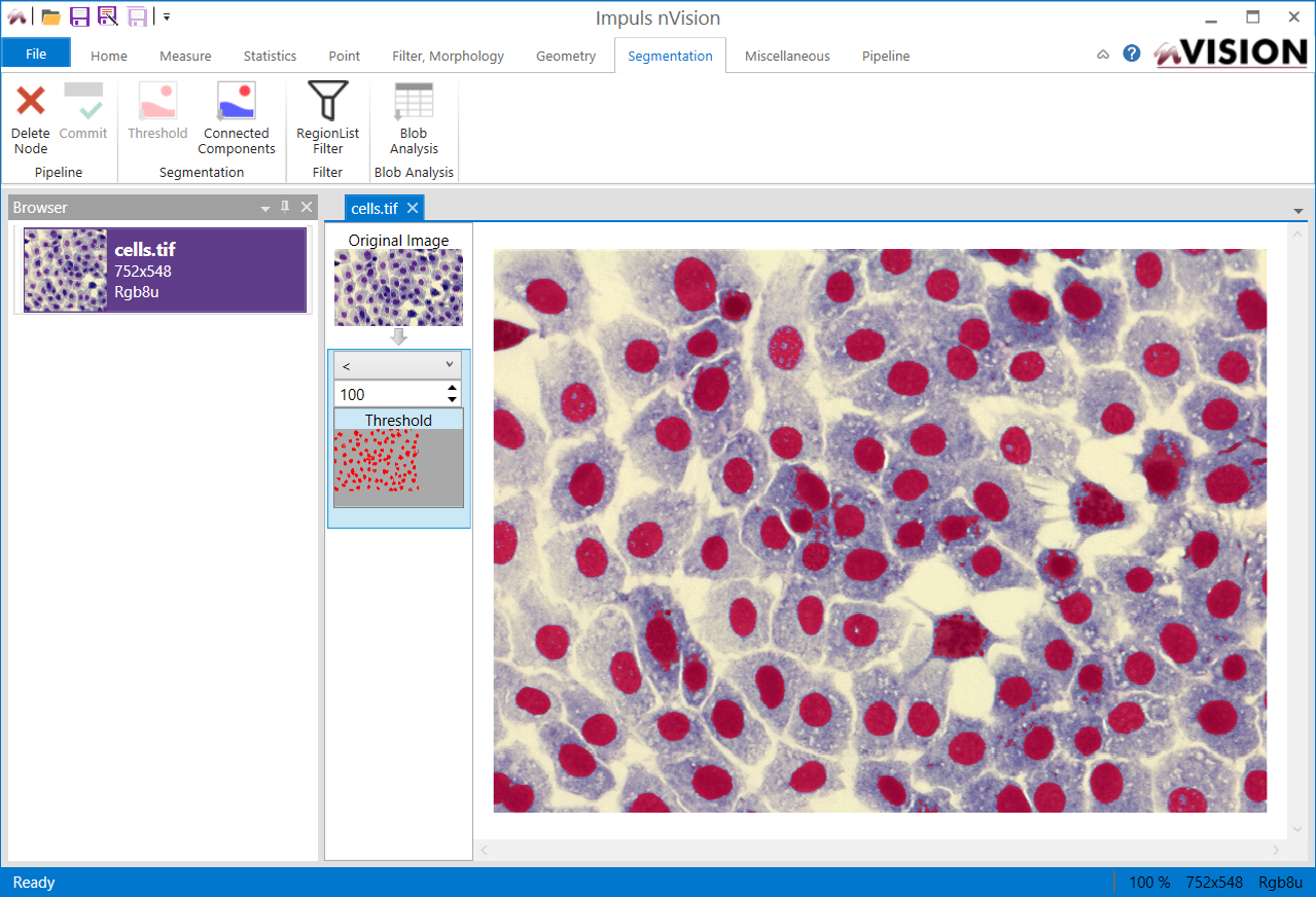
The result of the segmentation is overlaid in red on top of the image.
Of course you can change the thresholding mode as well as the threshold itself with the controls on top of the threshold node.
As a result of the thresholding, the appearance of the picture has changed, because the segmented cell nuclei are displayed in a red overlay color (partly transparent) on top of the original image. In addition, the threshold command has been appended to the linear processing pipeline, which now shows two steps.
3. Find connected components
From the Segmentation tab, use the Connected Components command.

Splitting a region into connected components.
This performs connected components analysis and splits the result from the previous segmentation step into connected objects.
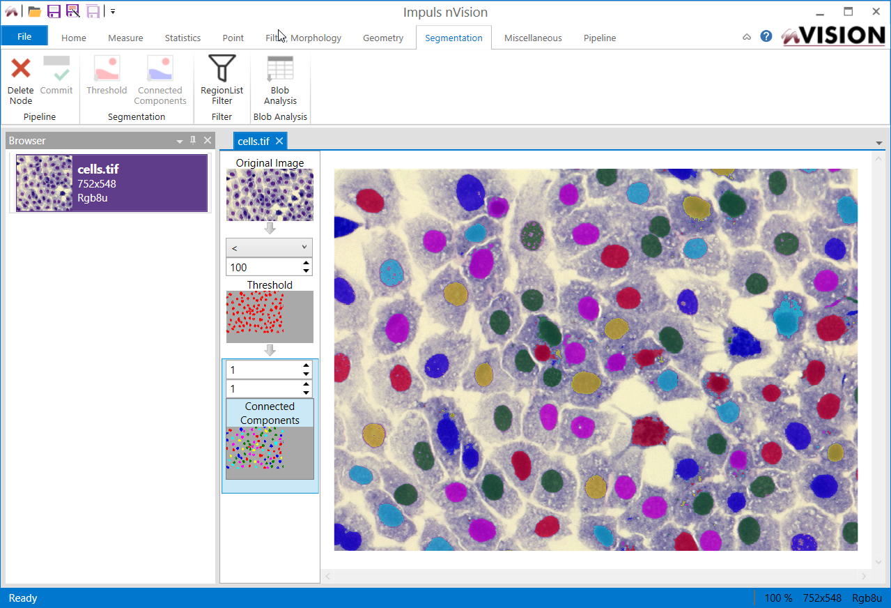
The result of the component splitting is overlaid on top of the image in color.
The appearance of the picture has changed again: now the different cell nuclei are displayed in different overlay colors. Also, the connected components command has been appended to the linear processing pipeline, which now shows three steps.
4. Analyze particles
The final step in our short introductory example is to analyze the particles.
From the Segmentation tab, use the Blob Analysis command.

Analyzing the blobs.
Now another step is appended to the pipeline displaying the total number of blobs, and a grid filled with numbers is displayed below the image.

The results of the blob analysis.
For each particle in the image, three is a row in the grid showing particle measurements (also sometimes called features). Between the image and the grid is a line with some checkboxes: Bounds and EquivalentEllipse. These are features that can be graphically visualized.
Make sure that you have either Bounds or EquivalentEllipse checked and click the Show checkbox in the first column of any grid row. This will show either the bounding box or the equivalent ellipse of said object in a graphical fashion.
You can also click the colored objects in the graphical view, and the grid scrolls to the line of the selected object.
In addition you can click the Commit button on the ribbon to commit the measurement results to the browser window. From there, the data can be exported to a CSV (comma separated values) file, which can be loaded into Excel or any other programs for further manipulation.
nVision has built a pipeline of commands as you have issued the commands. This pipeline can be re-used and applied to other images. In fact, you have built a little program, but you have done so without any programming. If you close nVision, this pipeline will be saved along the image (if the image is called cells.tif, the associated pipeline will be called cells.tif.xpipe).
We hope that this little tutorial has whetted your appetite for more and that you continue reading and working with nVision. Enjoy!